Technological features of power systems. Rated voltage scale for electrical installations
N The nominal voltage of a power transmission line significantly affects its technical and economic indicators. With a high rated voltage, high power can be transferred to long distances and with less losses. The power transmission capacity when moving to the next rated voltage level increases several times. At the same time, with an increase in the rated voltage, capital investments in equipment and construction of power lines increase significantly.
Rated voltages electrical networks GOST 21128 is established in Russia – 83 (Table 1).
Table 1
Nominal phase-to-phase voltages, kV,
for voltages above 1000 V according to GOST 721–77 (ST SEV 779–77)
| Networks and receivers | Generators and synchronous compensators | Transformers and autotransformers | Highest operating voltage | |||
| without on-load tap changer | with on-load tap-changer | |||||
| primary windings | secondary windings | primary windings | secondary windings | |||
| (3) * | (3,15) * | (3) and (3.15)** | (3.15) and (3.3) | – | (3,15) | (3,6) |
| 6,3 | 6 and 6.3** | 6.3 and 6.6 | 6 and 6.3** | 6.3 and 6.6 | 7,2 | |
| 10,5 | 10 and 10.5** | 10.5 and 11.0 | 10 and 10.5** | 10.5 and 11.0 | 12,0 | |
| 21,0 | 22,0 | 20 and 21.0** | 22,0 | 24,0 | ||
| – | 38,5 | 35 and 36.75 | 38,5 | 40,5 | ||
| – | – | 110 and 115 | 115 and 121 | |||
| (150) * | – | – | (165) | (158) | (158) | (172) |
| – | – | 220 and 230 | 230 and 242 | |||
| – | ||||||
| – | – | |||||
| – | – | |||||
| – | – | – | – |
* The rated voltages indicated in brackets are not recommended for newly designed networks.
** For transformers and autotransformers connected directly to the generator voltage buses of power plants or to generator terminals.
The economically feasible rated voltage of a transmission line depends on many factors, the most important of which are the transmitted active power and distance. The reference literature provides areas of application of electrical networks of different rated voltages, built on the basis of a criterion that is unsuitable in conditions market economy. Therefore, the choice of an electrical network option with a particular rated voltage should be made on the basis of other criteria, for example, the total cost criterion (see clause 2.4). However, approximate values of rated voltages can be obtained using previous methods (for example, using empirical formulas and tables that take into account the maximum transmission range and capacity of lines of different rated voltages).
The following two empirical formulas for determining voltage are most often used: U:
Or 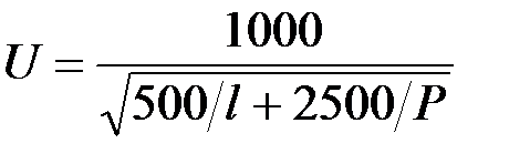 , (1)
, (1)
Where R- transmitted power, MW; l- line length, km.
The obtained voltages are used to select the standard rated voltage, and it is not at all necessary to choose a voltage that is always greater than that obtained using these formulas. If the difference in the total costs of the compared electrical network options is less than 5%, preference should be given to the option of using a higher voltage. The capacity and transmission range of 35–1150 kV lines, taking into account the most commonly used wire sections and the actual average length of overhead lines, are given in Table. 2.
Table 2
Capacity and transmission range of lines 35–1150 kV
| Line voltage, kV | Wire cross-section, mm 2 | Transmitted power, MW | Power line length, km | ||
| natural | at current density 1.1 A/mm 2* | maximum (at efficiency = 0.9) | average (between two adjacent substations) | ||
| 70-150 | 4-10 | ||||
| 70-240 | 13-45 | ||||
| 150-300 | 13-45 | ||||
| 240-400 | 90-150 | ||||
| 2´240-2´400 | 270-450 | ||||
| 3´300-3´400 | 620-820 | ||||
| 3´300-3´500 | 770-1300 | ||||
| 5´300-5´400 | 1500-2000 | ||||
| 8´300-8´500 | 4000-6000 | – |
* For overhead lines 750–1150 kV 0.85 A/mm 2.
Variants of the designed electrical network or its individual sections may have different nominal voltages. Usually, the voltages of the head, more loaded sections are determined first. Sections of the ring network, as a rule, must be run at the same rated voltage.
Voltages 6 and 10 kV are intended for distribution networks in cities, rural areas and industrial enterprises. The predominant voltage is 10 kV; 6 kV networks are used when enterprises have a significant load of electric motors with a rated voltage of 6 kV. The use of voltages of 3 and 20 kV for newly designed networks is not recommended.
The 35 kV voltage is used to create 6 and 10 kV power centers mainly in rural areas. In Russia ( former USSR) two voltage systems of electrical networks (110 kV and higher) have become widespread: 110–220–500 and 110(150)–330–750 kV. The first system is used in most IPS, the second after the division of the USSR remained only in the IPS of the North-West (in the IPS of the Center and the IPS of the North Caucasus, with the main system of 110-220-500 kV, 330 kV networks also have limited distribution).
Voltage 110 kV is the most widely used for distribution networks in all IPS, regardless of the adopted voltage system. 150 kV networks perform the same functions as 110 kV networks, but are available only in the Kola Energy System and are not used for newly designed networks. A voltage of 220 kV is used to create power centers for a 110 kV network. With the development of the 500 kV network, the 220 kV network acquired mainly distribution functions. The 330 kV voltage is used for the backbone of power systems and the creation of power centers for 110 kV networks. Backbone networks are operated at a voltage of 500 or 750 kV, depending on the adopted voltage system. For IPS, where a voltage system of 110–220–500 kV is used, a voltage of 1150 kV is accepted as the next stage.
Example 2
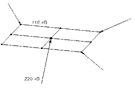
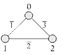
For the network development options selected in example 1 b, V And e(Fig. 1) select the rated voltages of network sections. Values of active loads at power points: R 1 = 40 MW, R 2 = 30 MW and R 3 = 25 MW.
Solution. All considered options are characterized by the presence of the head section of the network, CPU - 1. The power flow in this section of the network (without taking into account power losses in others) is equal to the sum of the loads of all three power nodes, i.e. R CPU – 1 = R 1 + R 2 + R 3 = 95 MW. According to expressions (1), we obtain voltages for this section of the network or 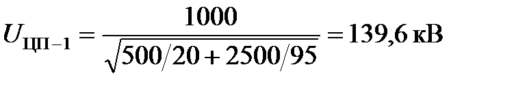 and, in accordance with the recommended voltage scale (Table 1), a nominal voltage of 110 or 220 kV can be accepted. Emergency current for a given section of the network at U n = 110 kV is equal to
 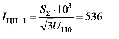 And, at U n = 220 kV – 268 kA. For both voltage classes, you can use the AC-240/32 wire grade in a 110 kV network according to permissible heating, in a 220 kV network - according to corona conditions. Let's consider the remaining sections of the designed network.
Section 1 – 2 is typical for all network development options b, V And e(Fig. 1) and differs in them only in the level of power flow through it. For option b voltages according to expressions (1) are respectively equal U 1 – 2 = 79.18 and U 1 – 2 = 96.08 kV, for options V And e U 1 – 2 = 92.14 and U 1 – 2 = 119.13 kV.
Section 1 – 3 is typical for two network development options – b And e. For option b the voltages for this section in accordance with expressions (1) are respectively equal to U 1 – 3 = 80 and U 1 – 3 = 91.29 kV, option e–U 1 – 3 = 97.43 and U 1 – 3 = 123.61 kV.
Section 2 – 3 is typical for options V And e. The voltages for this section are equal U 2 – 3 = 73.7 and U 2 – 3 = 92.59 kV.
Rated voltage values at the terminals of electrically connected products, including electric machines, established by GOST 23366-78. The requirements of this GOST do not apply to circuits closed inside electrical machines; on circuits that are not characterized by fixed voltage values, for example, on the internal power circuits of electric drives with engine speed control, and on the circuits of devices for reactive power compensation, protection, control, measurements, on the electrodes of cells and batteries. GOST numbers (ST SEV)
GOST 12.1.009-76 GOST 721-77 (ST SEV 779-77)
GOST 1494-77 (ST SEV 3231-81) GOST 6697-83 (ST SEV 3687-82)
GOST 6962-75
GOST 8865-70 (ST SEV 782-77)
GOST 13109-67 GOST 15543-70
GOST 15963-79 GOST 17412-72 GOST 17516-72 GOST 18311-80 GOST 19348-82
GOST 19880-74 GOST 21128-83
GOST 22782.0-81 (ST SEV 3141-81) GOST 23216-78
GOST 23366-78 GOST 24682-81 GOST 24683-81
GOST 24754-81 (ST SEV 2310-80)
Standards for specific groups and types of products containing voltage ranges, including GOST 21128-83, GOST 721-77, establishing rated voltages for power supply systems, source networks, converters and receivers electrical energy, are restrictive in relation to GOST 23366-78 and form a single set of standards with it.
GOST 23366-78 establishes the following nominal voltage values for products - consumers, sources and converters of electrical energy.
Rated voltages of consumers:
main series of voltages constant and AC, V: 0.6; 1.2; 2.4; 6; 9; 12; 27; 40; 60; 110; 220; 380; 660; 1140; 3000; 6000; 10000; 20000; 35000;
auxiliary AC voltage range, V:
1,5; 5; 15; 24; 80; 2000; 3500; 15000; 25000;
auxiliary voltage series DC, IN:
0,25; 0,4; 1,5; 2; 3; 4; 5; 15; 20; 24; 48; 54; 80; 100; 150; 200; 250; 300; 400; 440; 600; 800; 1000; 1500; 2000; 2500; 4000; 5000; 8000; 12000; 25000; 30000; 40000.
Rated voltages of AC electrical energy sources and converters, IN:
6, 12; 28,5; 42; 62; 115; 120; 208; 230; 400; 690; 1200; 3150; 6300; 10500; 13 800; 15 750; 18000; 20000; 24000; 27000; 38 500; 121000; 242000; 347000; 525000; 787000.
Rated voltages of DC electrical energy sources and converters, V:
6; 9; 12; 28,5; 48; 62; 115; 230; 460; 690; 1200; 3300; 6600.
For power sources of automotive and tractor equipment, the standard allows the use of rated voltages of 7V and 14V AC and 7V, 14V, 28V DC, as well as 36V AC with a frequency of 400 and 1000 Hz and 57V DC for power sources aircraft.
For short supply lines, the standard allows the rated voltage of sources and converters to be equal to the voltage of receivers.
The nominal values and permissible frequency deviations of power supply systems, sources, converters and electrical energy receivers directly connected to them, operating in steady state at fixed frequencies in the range from 0.1 to 10000 Hz, are established by GOST 6697-83. The specified GOST establishes the following main series nominal frequencies sources of electrical energy, Hz:
0,1; 0,25; 0,5; 1,0; 2,5; 5,0; 10; 25; 50; 400; 1000; 10000.
For converters and receivers of electrical energy, nominal frequencies, Hz, are selected from the range 0.1; 0.25; 0.5; 1.0; 2.5; 5.0; 10; 12.5; 16|; 50; 400; 1000; 2000; 4000; 10000.
For a number of special drives and their power sources, in particular for centrifuges, separators, woodworking machines, power tools, gearless electric spindles, electrothermal equipment, the standard allows the use of additional frequencies, Hz, from the range 100, 150, 200, 250, 300, 500, 600 , 800, 1200, 1600, 2400, 8000.
For aviation equipment, aircraft and their maintenance equipment, a frequency of 6000 Hz is allowed.
Permissible frequency deviations, % of the nominal frequency, are selected from the range 0.0002; 0.0005; 0.001; 0.002; 0.005; 0.01; 0.02; 0.05; 0.1; 0.2; 0.5; 1.0; 1.5; 2.0; 2.5; 5.0; 10 and are established in standards for specific types of sources, converters or power supply systems.
For general purpose networks, the standards for the quality of electrical energy at its receivers are established by GOST 13109-67. The standard establishes the following indicators of power quality:
- when powered from electrical networks single-phase current- frequency deviation, voltage deviation, range of frequency fluctuations, range of voltage changes, voltage non-sinusoidal coefficient;
- when powered from electrical networks three-phase current- frequency deviation, voltage deviation, amplitude of frequency fluctuations, amplitude of voltage changes, non-sinusoidality coefficient, asymmetry and voltage imbalance coefficients;
- when powered from DC electrical networks - voltage deviation, voltage variation range, voltage ripple coefficient.
INTERSTATE STANDARD "STANDARD VOLTAGES"
Standard voltages
Date of introduction 01/01/93
INFORMATION DATA
1. PREPARED AND INTRODUCED by the Technical Committee for Standardization TC 117 “Energy Supply”
2. APPROVED AND ENTERED INTO EFFECT by State Standard Resolution No. 265 dated March 26, 1992
3. This standard has been prepared by direct application method international standard IEC 38-83 "Standard voltages recommended by IEC" with additional requirements, reflecting the needs of the national economy
4. INTRODUCED FOR THE FIRST TIME
5. REFERENCE REGULATIVE AND TECHNICAL DOCUMENTS
6. REPUBLICATION. May 2004
This standard applies to:
Power transmission systems, distribution networks and power supply systems for alternating current consumers, which use standard frequencies of 50 or 60 Hz at a rated voltage exceeding 100 V, as well as equipment operating in these systems;
AC and DC traction networks;
DC equipment with a rated voltage below 750 V and AC equipment with a rated voltage below 120 V and a frequency (typically, but not limited to) 50 or 60 Hz. Such equipment includes primary or secondary batteries, other AC or DC power sources, electrical equipment (including industrial installations and telecommunications), various electrical appliances and devices.
The standard does not apply to the voltages of measuring circuits, signal transmission systems, as well as to the voltages of individual components and elements included in electrical equipment.
The a.c. voltages given in this standard are effective values.
This standard is used in conjunction with GOST 721, GOST 21128, GOST 23366 and GOST 6962.
The terms used in the standard and their explanations are given in the appendix.
Requirements that reflect the needs of the national economy are highlighted in bold.
1. STANDARD VOLTAGES OF AC NETWORKS AND EQUIPMENT
CURRENT IN THE RANGE FROM 100 TO 1000 V INCLUSIVE
Standard voltages in the specified range are given in table. 1. They refer to three-phase four-wire and single-phase three-wire networks, including single-phase branches from them.
Table 1
* The rated voltages of existing 220/380 and 240/415 V networks must be brought to the recommended value of 230/400 V. Until 2003, as a first step, electricity supply organizations in countries with a 220/380 V network must bring the voltages to value 230/400 V (%).
Electricity supply organizations in countries with a 240/415 V network must also adjust this voltage to 230/400 V (%). After 2003, a range of 230/400 V ± 10% must be achieved. The issue of lowering the limits will then be considered. All these requirements also apply to voltage 380/660 V. It must be reduced to the recommended value of 400/690 V.
**Do not use in conjunction with 230/400 and 400/690 V.
In table 1 for three-phase three-wire or four-wire networks, the numerator corresponds to the voltage between phase and zero, the denominator corresponds to the voltage between phases. If one value is specified, it corresponds to the phase-to-phase voltage of a three-wire network.
For single-phase three-wire networks, the numerator corresponds to the voltage between phase and zero, the denominator to the voltage between lines.
Voltages greater than 230/400 V are used primarily in heavy industry and large commercial buildings.
2. STANDARD VOLTAGES OF POWER SUPPLY SYSTEMS
ELECTRIFIED TRANSPORT POWERED BY CONTACT
DC AND ALTERNATING CURRENT NETWORKS
Standard voltages are given in table. 2.
Table 2
| Type of voltage contact network | Voltage, V | Rated frequency in alternating current network, Hz | ||||
| minimum | nominal | maximum | ||||
| Permanent | (400)* | (600) | (720) | |||
| 3600** | ||||||
| Variable | (4750) | (6250) | (6900) | 50 or 60 | ||
| 50 or 60 |
* In particular, on single-phase AC systems, the 6250 V nominal voltage should only be used when local conditions do not allow the 25000 V nominal voltage to be used.
The voltage values given in the table are adopted by the International Committee on Electric Traction Equipment and IEC Technical Committee 9 “Electric Traction Equipment”.
** In some European countries this voltage reaches 4000 V. Electrical equipment of vehicles involved in international traffic with these countries must withstand this maximum value for short periods of up to 5 minutes.
3. STANDARD VOLTAGES OF AC NETWORKS AND EQUIPMENT
CURRENT IN THE RANGE OVER 1 TO 35 kV INCLUSIVE
Standard voltages are given in table. 3.
Series 1 - voltages with a frequency of 50 Hz, series 2 - voltages with a frequency of 60 Hz. In one country, it is recommended to use only one of the voltage series.
The values indicated in the table correspond to phase-to-phase voltages.
Values in parentheses are not preferred. These values are not recommended when creating new networks.
Table 3
| Episode 1 | Episode 2 | |||
| Highest voltage for equipment, kV | Rated network voltage, kV | |||
| 3,6* | 3,3* | 3* | 4,40* | 4,16* |
| 7,2* | 6,6* | 6* | - | - |
| - | - | |||
| - | - | - | 13,2** | 12,47** |
| - | - | - | 13,97** | 13,2** |
| - | - | - | 14,52* | 13,8* |
| (17,5) | - | (15) | - | - |
| - | - | |||
| - | - | - | 26,4** | 24,94** |
| 36*** | 35*** | - | - | - |
| - | - | - | 36,5** | 34,5** |
| 40,5*** | - | 35*** | - | - |
* This voltage should not be used in general purpose electrical networks.
** These voltages usually correspond to four-wire networks, the rest - to three-wire networks.
*** Issues of unification of these values are considered.
In a series 1 network, the highest and lowest voltages should not differ by more than ±10% from the rated network voltage.
In a series 2 network, the maximum voltage should not differ by more than plus 5%, and the minimum - by more than minus 10% from the rated network voltage.
4. STANDARD VOLTAGES OF AC NETWORKS AND EQUIPMENT
CURRENT IN THE RANGE OVER 35 TO 230 kV INCLUSIVE
Standard voltages are shown in table. 4. In one country, it is recommended to use only one of those indicated in the table. 4 series and only one voltage from the following groups:
Group 1 - 123 ... 145 kV;
Group 2 - 245, 300 (see section 5), 363 kV (see section 5).
Values in parentheses are not preferred. These values are not recommended when creating new networks. The values given in table. 4, correspond to phase-to-phase voltage.
Table 4
In kilovolts
5. STANDARD VOLTAGES OF THREE-PHASE AC NETWORKS
WITH THE HIGHEST EQUIPMENT VOLTAGE EXCEEDING 245 kV
The highest operating voltage of the equipment is selected from the following range: (300), (363), 420, 525*, 765**, 1200*** kV.
_________________
*A voltage of 550 kV is also used.
**Voltages between 765 and 800 kV may be used, provided that the test values for the equipment are the same as those specified by IEC for 765 kV.
*** An intermediate value between 765 and 1200 kV, respectively different from these two values, will be included additionally if such a voltage is required in any area of the world. In this case, in the geographical area where this intermediate value is adopted, voltages of 765 and 1200 kV should not be used.
The series values correspond to the phase-to-phase voltage.
Values in parentheses are not preferred. These values are not recommended when creating new networks.
Group 2 - 245 (see Table 4), 300, 363 kV;
Group 3 - 363, 420 kV;
Group 4 - 420, 525 kV.
Note. The terms "region of the world" and " geographical area» can correspond to one country, a group of countries or part of a large country where the same voltage level is selected.
6. STANDARD VOLTAGES FOR EQUIPMENT WITH RATED
VOLTAGE LESS THAN 120 VAC AND LESS THAN 750 VAC
DC
Standard voltages are given in table. 5.
Table 5
| Nominal values, V | |||
| DC voltage | AC voltage | ||
| preferred | additional | preferred | additional |
| - | 2,4 | - | - |
| - | - | - | |
| - | - | - | |
| - | 4,5 | - | - |
| - | - | ||
| - | - | ||
| - | 7,5 | - | - |
| - | - | - | |
| - | - | ||
| - | - | ||
| - | - | ||
| - | - | - | |
| - | - | ||
| - | - | - | |
| - | - | - | |
| - | - | ||
| - | - | ||
| - | - | - | |
| - | - | - | |
| - | - | - | |
| - | - | ||
| - | - | - | |
| - | - | - | |
| - | - | - | |
| - | - | - | |
| - | - | - |
Notes: 1. Since the voltage of the primary and secondary batteries (batteries) is below 2.4 V and the choice of the type of element used for various applications depends on criteria other than voltage, these voltages are not listed in the table. The relevant IEC technical committees may specify element types and corresponding voltages for a particular application.
2. If technical and economic justification In specific areas of application, it is possible to use other voltages in addition to those indicated in the table. The voltages used in the CIS are established by GOST 21128.
APPENDIX 1
Information
TERMS AND EXPLANATIONS
| Term | Explanation |
| Rated voltage | The voltage to which the network or equipment is designed and to which its operating characteristics relate |
| Highest (lowest) network voltage | The highest (lowest) voltage value that can be observed in normal operation of the network at any point at any time. This term does not apply to voltage during transient processes (for example, during switching) and short-term increases (decreases) in voltage |
| Highest operating voltage of equipment | Highest value voltage at which the equipment can function normally indefinitely. This voltage is set based on its effect on the insulation and the equipment characteristics that depend on it. The highest voltage for equipment is the maximum value of the highest voltages of the networks in which this equipment can be used. |
| The highest voltage is indicated only for equipment connected to networks with a rated voltage above 1000 V. However, it should be borne in mind that for some rated voltages, even before this highest voltage is reached, it is no longer possible to carry out normal operation of the equipment from the point of view of such voltage-dependent characteristics, such as losses in capacitors, magnetizing current in transformers, etc. In these cases, the relevant standards must set limits under which normal operation of the devices can be ensured. | |
| It is clear that equipment intended for networks with a rated voltage not exceeding 1000 V, it is advisable to characterize only the rated voltage, both from the point of view of performance and insulation | |
| Consumer power point | The point in the distribution network of an electricity supply organization from which energy is supplied to the consumer |
| Consumer (electricity) | An enterprise, organization, institution, geographically isolated workshop, etc., connected to the electrical networks of the energy supply organization and using energy using electrical receivers |
As is known, the scale of rated voltages of electrical networks over 1000 V for general purpose alternating current is determined according to GOST 721-77 and recommends the following voltages for newly designed networks:
6, 10, 35, 110, 220, 330, 500, 750, 1150 kV.
When choosing voltage, it is necessary to take into account the existing voltage systems in the European part of Russia 110(150)/330/750 kV and in the Urals and Siberia - 110/220/500/1150 kV.
The voltage can be pre-selected using the empirical formula of G.A. Illarionova:
where is the line length, km; – power transmitted through the circuit, MW.
This formula gives satisfactory results for the entire scale of rated AC voltages in the range of 35–1150 kV.
There are other empirical formulas for choosing the nominal voltage. The scope of their application is limited to certain conditions presented below (Table 2.4).
Table 2.4
Formulas for selecting rated transmission voltage
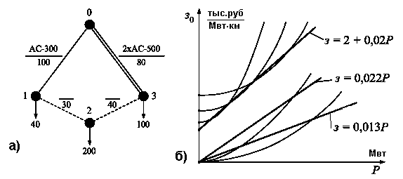
The areas of application of standard rated voltages depending on power and transmission range are shown in Figure 2.16 and Table 2.5.
Table 2.5
Power transmission capacity 110–1150 kV
| U nom, kV | F, mm 2 | Natural power, MW, at wave impedance, Ohm | Maximum transmitted power per circuit, MW | Maximum transmission length, km | ||
| 400 | 300–314 | 250–275 | ||||
| 70-240 | – | – | 25-50 | 50-150 | ||
| 240-400 | – | 100-200 | 150-250 | |||
| 2×240-2×400 | – | 300-400 | 200-300 | |||
| 3×330-3×500 | – | 700-900 | 800-1200 | |||
| 5×240-5×400 | – | – | 1800-2200 | 1200-2000 | ||
| 8×300-8×500 | – | – | 4000-6000 | 2500-3000 |
Today, the two systems that have developed in Russia have a rated voltage step within each approximately equal to 2 and a difference in transmitted power for adjacent voltages of 4–6 times. This leads to the fact that when transmitting a certain power, several circuits will be required at low voltage, and at high voltage the line will be underloaded. In this regard, when choosing a voltage, you can use U nom neighboring in the PUE, but with an increased splitting radius.
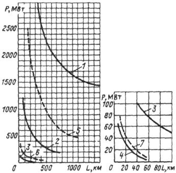
Rice. 2.16. Areas of application of electrical networks of different rated voltages. The limits of equal efficiency are indicated: 1 –1150 and 500 kV; 2 – 500 and 220 kV; 3 – 220 and 110 kV; 4 – 110 and 35 kV; 5 – 750 and 330 kV; 6 – 330 and 150 kV; 7 – 150 and 35 kV
Configuration
When choosing schemes for the development of electrical networks, the following techniques can be used:
A) reconstruction of the main transmission by adding a second circuit, sometimes at a higher voltage;

b) the emergence of new ring lines;
V) deep input at higher voltage.
Of course, the final choice of voltage and configuration should be based on technical and economic calculations.
Section selection
When choosing a cross-section, it is necessary to take into account the corona phenomenon, which determines the minimum permissible cross-section for each rated voltage.
The maximum permissible cross-section for power transmission lines depends on the rated voltage and is determined by the rational ratio of the consumption of non-ferrous and ferrous metal in the line structure.
The cross section is selected according to economic current density or economic intervals. Economic density is determined by the minimum cost in power transmission lines and depends on the type of line, wire material, and load schedule.
2.8.2. Economic intervals
The use of economic intervals makes it possible to exclude discrete sections and rated powers of transformers from the number of variables. Using economic intervals, it is possible to present costs as a function of only the transmitted power. When choosing the structure of generating capacities, costs in power transmission lines can be presented in the form. When planning network development, you can use a more accurate approximation in the form ![]() or
or ![]() , but they all have a gap at . An approximation of the form can be used as a continuous function
, but they all have a gap at . An approximation of the form can be used as a continuous function ![]() , according to which at costs
, according to which at costs ![]() can be reduced by selecting ε.
can be reduced by selecting ε.
When choosing economic intervals for transformers, costs are taken into account by the following formula:
where is the cost of the th transformer; – transformer operating time;
– the cost of lost energy, determined by the costs of basic ES;
– cost determined by costs at peak stations.
Usually, but often taken ![]() .
.
From the condition ![]() the upper limit of the economic interval of the transformer is determined with rated power.
the upper limit of the economic interval of the transformer is determined with rated power.
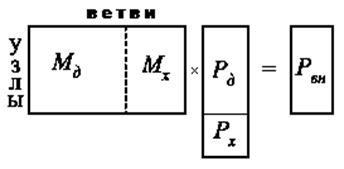
2.8.3. Mathematical model for network development planning
The formation of a model begins with drawing up a calculation diagram, which shows existing nodes and branches, new nodes and possible additional routes of lines connecting objects into the system. Here, those lines that were found as a result of analyzing the model for choosing the structure of generating capacities should also be taken into account. The design scheme must be reasonably redundant and include additional lines so as not to miss possible optimal connections.
For nodes, predicted loads and powers of input blocks must be specified. Thus, the design scheme will have design nodes, including existing ones; those. node index ![]() . The number of branches in the design scheme, of which are existing.
. The number of branches in the design scheme, of which are existing.
Active power flows along the branches can be taken as unknowns ![]() .
.
As an objective function, consider the costs in existing lines, proportional to energy losses, and into new lines, determined in accordance with the accepted approximating expressions for costs:
 , (2.35)
Where  .
.
The unknown power flows along the branches are subject to the power balance condition at the nodes, which can be written in matrix form:
![]() .
.
– rectangular matrix of node-branch connections, with its elements for node and branch s are denoted and can take values equal to 1 if the branch leaves the node; +1 if the branch is included in the node and 0 if it is not connected to the node.
Let's create a balance equation for the node (Fig. 2.19):
IN general view The balance equation for any node can be written:
![]() .
.
Thus, the task of choosing the optimal network design is to find the minimum of some nonlinear function ![]() subject to a linear constraint in the form of equality
subject to a linear constraint in the form of equality ![]() .
.
The problem of network development planning formulated in this way is reduced to a nonlinear programming problem. This problem, as a rule, has one extremum. To solve it, the previously discussed nonlinear programming methods can be used.
2.8.4. Application of gradient methods
As is known, the basic equation of the gradient method is:
![]() . (2.36)
. (2.36)
Let's consider an example in which it is necessary to select a network to power only one node (Fig. 2.20). We believe that costs are represented by quadratic dependencies. As a starting point we take R 0 =(0,R N).
When taking into account restrictions, the movement to the minimum should be carried out according to the projection of the gradient onto the surface of the restrictions, i.e. along the vector V. Vector V can be obtained by eliminating the constraints from the components perpendicular to the surface. These components form a gradient of constraints. So the vector V determined by the expression
![]() . (2.37)
. (2.37)
To determine the undetermined factors forming the vector V, the condition for the scalar product to be zero is used:
. (2.38)
From this condition, taking the gradient for the linear constraint to be equal to , we can find . Indeed, from the transformation
we can obtain the following matrix expression for the factors
![]() . (2.40)
. (2.40)
Components of the multiplier vector λ allow you to determine all components of the vector V
 ,
,
and use them in the gradient method procedure
![]() .
.
However, it is easier to find the gradient projection if you substitute expression (2.40) in (2.37) and carry out a simple transformation
Where P=![]() - design matrix.
- design matrix.
The iterative process continues until the required accuracy condition for all components is met.
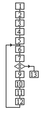 Rice. 2.21 Rice. 2.21 | A block diagram of the algorithm with the selection of the optimal step is shown in Figure 2.21. Purpose of the blocks: 1. Formation of the calculation scheme. 2. Determining the type of functions for calculating costs and their derivatives for all branches. 3. Formation of the incidence matrix M. 4. Determination of the gradient design matrix P. 5. Initial approximation of flows P = P0. 6. Calculation of the gradient at point P. 7. Definition of projection V gradient. 8. Checking the end condition. 9. Organization of a trial step P 1 = P- V t 0/ . 10. Gradient and Projection Calculation V 1 at the end of the step. 11. Determining the optimal step |
Example 2.3. Determine the optimal flows in the branches of the network, the design diagram of which is shown in Figure 2.22.
Iterative calculation begins by accepting the initial approximation P 0, determining the magnitude of the gradient and projecting it onto the constraint surface
Then a tentative step is taken in the direction of the projection t 0 =0.1 and flows are determined along branches P 1 at the end of this step, the gradient and its projection
After this, you can determine a step close to the optimal one
and perform a working step from the starting point P in the direction of projection
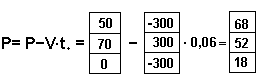
After this, in accordance with the algorithm, we return to block 6, where the gradient and its projection are again calculated
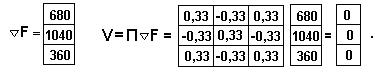
Checking the condition in block 8 determines the completion of the iterative process.
Based on the flows found, you can select the cross-section of the power line.
The rapid convergence of the process is explained by the quadratic nature of the objective function, which has a linear gradient and the optimal step found from two points leads to an exact solution.
The disadvantage of the method is the large dimension of the problem, determined by the number of branches of the calculation scheme.
2.8.5. Coordinate optimization method
In a design scheme, as a rule, the minimum is the number of circuits, defined as the difference in the number of branches and nodes. Therefore, when optimizing, it is advisable to use contour powers as unknowns and apply the coordinate-wise search method. The advantage of this method is that at each step of optimization of the objective function ![]() Only one variable is selected with the remaining values fixed. The found value is fixed, and then they move on to optimizing the next variable, etc.
Only one variable is selected with the remaining values fixed. The found value is fixed, and then they move on to optimizing the next variable, etc.
Consider the balance constraint. All flows along branches can be divided into two components:
![]() ,
,
where are the flows in the tree, the branches of which connect all nodes with the balancing one without forming contours;
–flows in chords, i.e. in the branches forming the contours.
The basic constraint can be thought of as divided into block matrices, as shown in Figure 2.23.
The flows in the branches of the tree are uniquely determined by the flows in the chords, which follows from the relations obtained based on operations with block matrices and presented below:
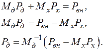 (2.42)
As an initial approximation we can take:
Then the streams in the trees:
![]() .
.
Different branches of the original circuit can be selected as chords, complementing the selected tree to form contours. The number of combinations is determined by the possible number of trees, calculated using the Trent determinant generated for independent nodes:
 , (2.43)
where is the number of branches associated with the node; – the number of branches connecting nodes and .
Example 2.4. Determine the number of trees for the diagram
 |  |
Contour optimization is carried out according to the following algorithm.
1) A calculation scheme is drawn up.
2) Dependencies are determined to account for costs in the line of the calculation scheme. For this purpose, any approximating functions can be used up to the exact lower envelope of the costs of new lines.
3) The chords for which the initial flow approximation is accepted are selected and numbered, and the flows in the branches of the tree are counted.
4) A cycle is organized along chords, in which the following operations are performed sequentially:
– for the current chord, the contour that it closes is viewed;
– based on the received flow in the chord, the flows in the branches of the circuit are determined;
– for flows in the branches of the circuit, the costs in each branch and the total costs in all branches of the circuit are calculated;
– sequentially changing the value of the chord flows in the direction of increasing or decreasing, while new flows in the branches of the circuit and new costs are determined, which are compared with the previous ones until the minimum is found.
Thus, optimization is carried out. If costs are calculated by approximation , then we can consider flows in a chord at which a branch with zero power appears in the circuit, which ensures minimum costs. After this, the current chord is transferred to this branch.
5) After exiting the cycle, the new position of the chords is compared with the previous one. If it does not match, then another optimization cycle is carried out. If there is a match, the calculation ends. Usually two or three cycles are enough.
Example 2.5. Choose optimal plan development of the 220 kV network, which is presented in Figure 2.25-a.
For the network under consideration, development is associated with an increase in loads and the connection of a new substation. The dotted line shows possible power line routes. Figure 2.25-b shows the cost curves for existing and new power lines and their linear approximations.
The table shows expressions for determining the costs of each branch of the design scheme, taking into account the length.
Table 2.6
| Line | Cost |
| 0-1 | |
| 1-2 | |
| 2-3 | |
| 0-3 |
There is only 1 contour in the design scheme and we will take section 2-3 as the initial position of the chord. Let's select all branches of the circuit to calculate costs. The iterative process is presented in Table 2.7:
Table 2.7
| 0-1 | ||||||
| 1-2 | ||||||
| 2-3 | ||||||
| 0-3 | ||||||
In the initial position of the chord, the costs amounted to 812 thousand rubles. Moving the chord to an adjacent position changed the flows and reduced costs. Further movement in the same direction turned out to be no longer profitable.
As a result of optimization, a tree corresponding to the minimum cost is found.
For a network of any complexity, the iterative process converges quite quickly. In this case, special fast algorithms used for open-loop networks can be used. They are based on the "second address mapping" method.
The tree found as a result of optimization determines the basis of the developing network, which can be supplemented taking into account the requirements of reliability and quality of the mode.
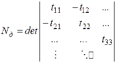
Let us consider the essence of the method of second address mappings, which can be used when choosing the optimal tree of a developing network. Let's consider an open circuit (Fig. 2.26), in which the load is supplied from the power center to several consumers. For given nodal loads, for example current, the current of each branch is determined by simply summing the currents of those nodes that pass through this branch. If the network diagram is specified in pairs of nodes for each branch strictly in the direction from the CPU, which is quite natural, then the serial number of the starting node of the branch in the list (array) of end nodes will make it easy to organize a passage from any node to the CPU, which must have a special path to complete the path number, for example negative. The numbers found in this way for each branch are called “second addresses”.
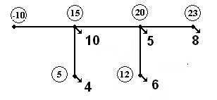
Table 2.8
| Item no. | UN | UK | THAT | UN2 | Branch current (TV) |
| -10 | -10 | 10+4+6+8+5=33 | |||
| 5+4+8=17 | |||||
The table shows the initial data and stages of calculating the branch currents. Array designations here: UN – start nodes, UK – end nodes of branches, TU – node currents, TV – branch currents, UN2 – second address mappings.
When analyzing the table, you should pay attention to the fact that with a correctly specified network configuration, each node number in the UN array can be found in the UK array. As already noted, its place, i.e. the sequence number in this array is called the second address mapping.
The found addresses can be used to determine branch currents, power flows, losses, i.e. to calculate the mode. Let us consider the procedure for determining currents by branches. Here, first, all elements of the TU array are rewritten into the TV array, and then the currents of all nodes, starting from the last one, are superimposed by summing on the currents of the branches through which the node is powered from the power point in accordance with the second addresses.
The calculation of power flow distribution, taking into account power and voltage losses is carried out in a similar way.
Let's consider two algorithms used in the analysis of open-loop networks.
Figure 2.27 shows a block diagram of the algorithm for determining second addresses, and Figure 2.28 shows a block diagram of the algorithm for calculating current distribution.
In the contour optimization algorithm of a developing network, the chords are combined into a separate array, where second addresses are formed for both nodes of the open branch. In the optimization cycle, a power node is determined for each chord, which acts as a CPU and limits the movement of the chord position in the one-dimensional optimization process.
2.8.6. The branch and bound method (BMB) for choosing the optimal
distribution network
Distribution networks, as a rule, are operated in open circuits. The basis for selecting a new network is to find the minimum cost tree. The number of possible trees is huge and will be determined by Trent's determinant. The optimal tree can be found by calculating the costs for each tree out of the entire set of possible trees. But such viewing of all combinations is not realistic even with modern computers.
The essence of the branch and bound method is to split the entire set of possible plans into subsets, followed by a simplified assessment of the effectiveness of each and discarding (excluding from further analysis) unpromising subsets. In essence, this is a combinatorial method, but with a targeted enumeration of options. The method first appeared in 1960 to solve a linear integer programming problem, but went unnoticed, and only in 1963 was it effectively used to solve the problem of a traveling salesman who must travel around all commercial points along the shortest route. Orienteering athletes also solve a similar problem.
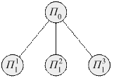
The original set and all current ones are divided into disjoint subsets, where is the partition number, and is the serial number of the subset at the partitioning stage (Fig. 2.29).
For the original set, there is an unknown plan with minimal cost
![]() , (2.44)
, (2.44)
where is the exact lower limit of costs, which is unknown;
is the exact lower bound on costs, which also exists for .
We believe that there is a possibility for a fairly simple determination of some external cost estimate for this subset, for which the condition is satisfied. This estimate can be used to identify “expensive” subsets that can be excluded from further partitioning. To increase reliability in competitive subsets, internal estimates are also considered, for which. External and internal assessments are shown in Figure 2.30.
Promising subsets are divided similarly. The branching process continues until there are several options left in the subset (2÷4) or the external and internal estimates = coincide.
Let us consider the application of the idea of the branch and bound method for the problem of searching for a new distribution network with linear approximation of costs in the branch of the calculation scheme
Russia
In Russia, two series of nominal voltages have been developed, which include both ultra-high and ultra-high voltage lines. The first scale is 110-150-330-750 kV, the second is 110-220-500-1150 kV.
Each of the subsequent steps in these scales exceeds the previous one by approximately 2 times, which makes it possible to increase the transmission capacity by approximately 4 times.
These voltage scales have their own application areas. The first scale has become widespread in the North-Western regions of Russia, Karelia, the Kola Peninsula and the North Caucasus. The connections between the integrated system of the North-West and the Kola Energy System are made at a voltage of 330 kV, the IPS of the North-West with the IPS of the Center - at a voltage of 750 kV.
The second voltage scale is used in the Center of Russia and regions located east of Moscow. In the Central Zone, the two scales mentioned sometimes overlap (500 and 750 kV lines). At the same time, east of Moscow, including Siberia and the Far East, only the second voltage scale is used. This division of two scales into different territories has its advantages from the point of view of network operation.
USA
The first power transmission lines with a voltage of 110 kV were built in the USA back in 1910, 220 kV - in 1922. Then a number of other nominal voltages appeared, which is due to a large number companies producing electrical equipment. In the 50s, 345 kV lines were developed, in 1965 the first 500 kV line was turned on, in 1969 - a 765 kV line, and in 1970 a ±400 kV DC power transmission line with a length of 1400 km came into operation ( Pacific transmission), passing along the west coast of the United States. Despite the variety of nominal voltages in this country, two scales can be distinguished that have their own areas of application. The first scale includes voltages of 138-345-765 kV and is used in the Southwest, Center and North of the country, the second - voltages of 115-230-500 kV and is used mainly in the West and South-East of the United States.
In the United States, there are a number of interconnected energy systems, which include individual energy companies, of which there are more than thousands. Some of these consolidations are controlled from a single control center, others simply operate in parallel while coordinating load sharing and frequency regulation. The role of intersystem connections and system-forming lines is performed by 345-765 kV lines. Work is underway to create equipment for 1600 kV power lines.
In the north, the US power grid has strong connections to Canada, including several 765 kV lines in the eastern part of the border, several 500 kV lines in the western part, and three DC insertions.
In the 90s of the last century, a multi-substation DC power transmission Canada-USA (1486 km, ±400 kV, 2000 MW) was built from the La Grande hydroelectric station in the province of Quebec (Canada) to Boston (USA). This transmission has five converter substations, three of which are located in Canada and two in the United States. In addition to this transmission line, there are three more transmission lines and eight DC insertions in the United States.
In the south, the US power grid is connected by 230-345 kV lines to the Mexican power grid. The power systems of Canada, the United States and Mexico operate in parallel.
Western Europe
In Western Europe, there is an energy association UCPTE, which includes 12 countries, to which countries are now also connected Eastern Europe. The Nordic countries have created the Nordel System energy association, which includes Sweden, Norway, Finland and Denmark. The Anglin grid operates in parallel with the UCPTE via a subsea DC transmission line. Similar transmission lines also connect the power systems of Sweden, Denmark and Germany with the power systems of Sweden and Finland. Russia is connected to the Nordel System through a DC link in Vyborg with a capacity of 1420 MW. It is planned to build a 724 km long UK-Norway submarine DC line with a capacity of 800 MW.
The main system-forming alternating current lines in Western European countries that are members of the UCPTE are lines with a voltage of 380-420 kV. 230 kV lines and 110-150 kV lines perform the functions of distribution networks. Voltages of 500 and 750 kV are not used in Western Europe, but in France, due to increasing loads, a project for the construction of 750 kV lines has been developed. In this case, it is proposed to use newly constructed 380 kV lines with two wires in phase on double-circuit supports to suspend one 750 kV circuit with the same wires.
Canada
In the eastern part of the country, a network with a voltage of 735 kV is quite widely developed, in the western part - 500 kV. The development of the 735 kV network was caused by the need to provide power to one of the world's largest hydroelectric power stations on the river. Churchill with a capacity of 5.2 GW, as well as a cascade of hydroelectric power stations on the river. St. Lawrence. To supply power from hydroelectric power stations on the river. Nelson built the Nelson River - Winnipeg DC power line - a double-circuit transmission 800 km long: the first circuit on mercury valves (±450 kV, 1620 MW), the second circuit on high-voltage thyristor valves (±500 kV, 2000 MW). In addition, there is a 320 MW Il River DC link designed to connect the power systems of Canada and the United States. On the West Coast
Canada has laid an underwater transmission from the mainland to the island. Vancouver, which has two AC cables (138 kV, 120 MW) and two DC cables (+260+280 kV, 370 MW). There is also a Shategei DC link (1000 MW), linking the 735 kV network in Canada and the 765 kV network in the USA.
The developed 500 kV networks in western Canada connect large power plants and load nodes in industrial areas of the western provinces. The power systems of the eastern and western parts of Canada do not have a direct connection, since they are separated by mountain ranges. Communication is carried out through the US power grid. There are 500 kV interconnections between the Canadian and US grids in the western portion of those countries.
Thus, in the northern USA and southern Canada there are two large energy interconnections: the energy systems of the northeastern part of the USA and the southeastern part of Canada and the energy systems of the northwestern part of the USA and southwestern Canada.
Mexico, Central and South America
Mexico's power grid has disproportionately less capacity than the US power grid. The main network in Mexico is formed at voltages of 220 and 400 kV.
The countries of Central America (Panama, Costa Rica, Honduras, Nicaragua) form an energetically isolated region with a small total power plant capacity (3-4 GW). There are 230 kV interstate connections. Currently, the Central American Energy Association is being created on the basis of the construction of 230-500 kV lines.
Among the countries South America Brazil (54%), Argentina (20%) and Venezuela (10%) have the most powerful energy potential. The rest comes from other countries on the continent. At the same time, Argentina's energy system is the largest in South America. The highest network voltage in Argentina is 500 kV, the total length of lines of this voltage class is about 10 thousand km.
The highest voltage of electrical networks in Brazil is 765 kV. There is also a network of 500 kV lines, separate lines of 400 kV and a network of 345 kV. In Brazil, a direct current power transmission line is operated from the world's largest hydroelectric power station, Itaipu, to the Sao Paulo area. This power transmission has two voltages of ±600 kV, its length is over 800 km, and the total transmitted power is 6300 MW.
The highest network voltage in Venezuela is 400 kV. In other countries of this continent - 220 kV. There are a number of 220 kV interconnections.
Wide interconnection of South American electricity systems is hampered by the different nominal frequencies of individual countries: 50 and 60 Hz. There are two DC inserts. One of them is with a capacity of 50 MW between the networks of Paraguay and Brazil, the other with a capacity of 2000 MW between the networks of Brazil and Argentina.
Africa
Given the large area of the continent, the total power of power plants is relatively small. Of these, approximately half are concentrated in South Africa and over 10% in Egypt, the rest in other countries of the continent. With relatively modest energy capacities, African energy systems use fairly high voltages, which is explained by the remoteness of energy sources from consumption centers. In Egypt, the voltage used is 500 kV, in South Africa - 400 kV, Nigeria, Zambia and Zimbabwe - 330 kV, in other countries 220-230 kV. Two powerful direct current power lines have been built on the continent: Inga - Shaba, connecting the two most developed but isolated regions of Zaire, and the Cabora Bassa (Mozambique) - Apolo (South Africa) hydroelectric station.
Asia (excluding CIS)
For this region, due to the lack of sufficiently complete information, only the most general information. The highest voltage of system-forming lines in India, Turkey, Iraq, Iran is 400 kV, in China, Pakistan, Japan - 500 kV. In India and China, much attention is paid to power transmission and DC insertions. In these countries, several power transmission lines and direct current inserts have already been built and it is planned to increase their number and carry out all intersystem connections on direct current.
Among Asian power systems, the leading positions are occupied by the power systems of Japan and South Korea. The backbone of Japan's backbone network is 275 and 500 kV lines. Almost all 500 kV lines are double-circuit. To transmit electricity to the Tokyo area from a large nuclear power plant, a 1100 kV power transmission line with a length of 250 km was built. This line is built on double-chain supports up to 120 m high, which is determined by environmental requirements. Currently, construction of a 1100 kV ring line is underway on the island. Honshu.
The difficulty in creating a unified energy system in this country is the presence of different nominal frequencies (50 and 60 Hz) in the northern and southern parts Japan. The border between these parts runs along the island. Honshu. For communication between them, two 300 MW DC inserts were built. In addition, the two islands - Hokkaido and Honshu - are connected by overhead cable DC power transmission (600 MW, ±250 kV).
Backbone network South Korea has a voltage of 345 kV. Due to the small size of the territory of this state, power lines are short in length. The total length of 345 kV lines running in the meridional direction is slightly more than 300 km. The total length of lines running in the latitudinal direction is approximately the same. The routes of these lines, as a rule, pass through areas not affected by economic activity, which in the conditions of South Korea is very difficult. Due to the increase in load, a 765 kV line is being built, which also requires overcoming difficulties with laying the route.
The main features of power systems are the following.
Electricity is practically not accumulated. Production, transformation, distribution and consumption occur simultaneously and almost instantly. Therefore, all elements of the energy system are interconnected by the unity of the regime. In the power system, at each moment of time in a steady state, a balance is maintained in the active and reactive power. It is impossible to produce electricity without a consumer: how much electricity is generated in at the moment, so much of it was given to the consumer minus losses. Repairs, accidents, etc. lead to a decrease in the amount of electricity supplied to the consumer (in the absence of a reserve), and, as a consequence, to underutilization of the installed power system equipment.
Relative speed of processes (transient): wave processes - () s, switching off and turning on - s, short circuits- () s, swings - (1-10) s. High flow rates transient processes in energy systems necessitate the use of automation within a wide range, up to the complete automation of the process of production and consumption of electricity and the exclusion of the possibility of personnel intervention.
The power system is connected to all sectors of industry and transport, characterized by a wide variety of electricity receivers.
Energy development must outpace the growth of electricity consumption, otherwise it is impossible to create power reserves. Energy should develop evenly, without disproportions of individual elements.
Advantages of interconnecting power plants into a power grid
When combining power plants into an energy system, the following is achieved:
reduction of the total power reserve;
reduction of the total maximum load;
mutual assistance in case of unequal seasonal changes in power plant capacity;
mutual assistance in case of unequal seasonal changes in consumer loads;
mutual assistance during repairs;
improving the capacity utilization of each power plant;
increasing the reliability of power supply to consumers;
the possibility of increasing the unit capacity of units and power plants;
possibility of a single control center;
improving the conditions for automating the process of production and distribution of electricity.
Electrical installations. Nominal installation data
Electrical installations (PUE, I.1-3) - installations in which electricity is produced, converted, distributed and consumed. They are divided into electrical installations with voltages up to 1000 V and over 1000 V.
The rated (PUE, I.1-24) current, voltage, power, power factor, etc. of an electrical installation are the passport data (in practice, these are the data at which the operation of the electrical installation is most economical).
Rated voltages
The scale of nominal voltage lines in kilovolts for electrical installations of three-phase alternating current with a frequency of 50 Hz is given in table. 1.
Table 1
Scale of rated voltages of electrical installations, kV
|
Electrical receivers |
Generator |
Transformer |
|
|
primary winding |
secondary winding |
||
The rated voltage scales of generators and secondary windings of transformers are chosen to be 5-10% higher than the rated voltages of consumers, power lines, and primary windings of transformers in order to facilitate maintaining the rated voltage of consumers.
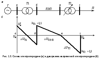
The reference base is the rated voltage of the consumer (), then the rated voltage of the generator, the secondary winding of the transformer. With the help of rationally selected rated voltages and transformation ratios, it is possible to compensate for the voltage drop in the power transmission (,,) and maintain the rated voltage for the consumer.
The maximum permissible operating voltages exceed the rated voltages by 15%(), 10%() and 5%().
Maximum voltage scale, kV: 3.6; 6.9; 11.5; 23; 40.5; 126; 172; 252; 525; 787; 1207.5.
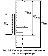
Changing the transformation ratio is achieved by changing the number of turns (tap) on one of the windings, for example, when and,
This expression means that the number of turns changes on the side high voltage from to, while changing from to (Fig. 1.4):
Review information about transformers given in electrical reference books and determine the limits and stages of regulation of transformation ratios.